Aggregate Window Functions

Last time out we talked about the Ranking options which are available for Window Functions. This time we’ll be covering the Aggregate options which are available to us with them. We’ll also introduce a new feature to see how we can limit the rows the function is performed on, but different to the PARTITION method.

For this we’ll be using the same sample data which we started with previously:

CREATE TABLE #QuarterlySales (
	FinancialYear CHAR(6),
	FinancialQuarter CHAR(6),
	QuarterlySales INT
);

INSERT INTO #QuarterlySales
VALUES ('FY2020', '2020Q3', 1), ('FY2020', '2020Q4', 2),
	('FY2021', '2021Q1', 4), ('FY2021', '2021Q2', 8),
	('FY2021', '2021Q3', 16), ('FY2021', '2021Q4', 32),
	('FY2022', '2022Q1', 64), ('FY2022', '2022Q2', 128),
	('FY2022', '2022Q3', 256), ('FY2022', '2022Q4', 512),
	('FY2023', '2023Q1', 0);

An aggregate example

Lets jump straight into an example of the aggregate options which are on offer. Now unlike the ranking functions where we needed to use the ORDER BY clause in the function, that’s not necessarily the case for aggregates. Below we’ll use the SUM function with just a partition applied:

SELECT *,
	SUM(QuarterlySales)
		OVER (PARTITION BY FinancialYear)
		AS [YearlySales]
FROM #QuarterlySales;

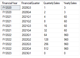
Now we’re applying a sum with the scope limited to each financial year so we’ll get a side by side of the quarterly and yearly totals. With your own dataset you could implement something similar to provide daily, weekly, monthly and annual sales all from the same set of results for example.

There’s quite a list of functions which are listed in the documentation for the aggregate functions. Below are a selection of the more common ones which are used and you can find the full details for these and others in the documentation:

• AVG – the average value within the range
• COUNT – the count of elements in the range (returns type INT)
• COUNT_BIG – the count of elements in the range (returns type BIGINT)
• MAX – the largest value across the range
• MIN – the smallest value across the range
• SUM – the total value across the range

The ordering difference

When we looked at the ranking functions the ordering was key in their results and was therefore mandatory. This isn’t the case with the aggregates, however using an ORDER BY can bring some benefits – let’s see what that looks like. We’ll try the same thing again but this time we’ll specify the ordering to be based on the quarter to see what that changes:

SELECT *,
	SUM(QuarterlySales)
		OVER (PARTITION BY FinancialYear
		ORDER BY FinancialQuarter)
		AS [YearToDateSales]
FROM #QuarterlySales;

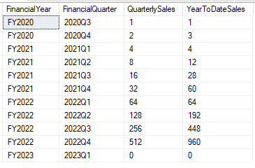
Well that’s pretty cool, we end up with a rolling SUM applied across a partitioned data set!

This is one of the powerful features of the aggregate window functions. Without the ability to do this, rolling calculations like these can require self joins and some tricks, particularly if you’re looking to perform multiple of them in a single result set. As we’ve saw last time, it’s not to say that these functions are without cost, however they do make reading and understanding queries much more straightforward than they may be if the same result were hand-crafted.

Limiting the scope

Whilst we’re on a roll (pun intended, I’m sorry) its a good time to look at another way we can extend Window Functions by using the ROWS keyword to limit the scope of the function. We already have the PARTITION to allow us to limit the scope relative to something within the data however the ROWS allows us to operate relative to the rows in the results. If we wanted to create a year to date as above we could use the ROWS expression to provide the same result:

SELECT *,
	SUM(QuarterlySales)
		OVER (PARTITION BY FinancialYear
		ORDER BY FinancialQuarter
		ROWS BETWEEN UNBOUNDED PRECEDING
			AND CURRENT ROW)
		AS [YearToDateSales]
FROM #QuarterlySales;

Well that’s a little bit of new syntax right there! Lets work through this and explain what we’ve got here:

• ROWS BETWEEN – this indicates that we’re limiting the ROWS where we want the function applied and we’re using BETWEEN since we’re specifying the start and end of the range. If we only specify one of these then we can drop the BETWEEN and the range will either start or end based on the current record
• UNBOUNDED PRECEDING – here we’re saying we want to apply the SUM against all records prior to this one, but whilst still being within the same partition. For example the record for quarter 2021Q3 would also cover 2021Q1 and 2021Q2 as they’re prior to Q3 (based on the ORDER BY) and still within the same Financial Year (adhering to the PARTITION)
• AND CURRENT ROW – we want the range to end at the current row in the sequence, so as in the example above we’ll stop the SUM function at Q3 and ignore any of the Q4 sales

In addition to the ability to specify rows PRECEDING we can also define the rows FOLLOWING if we want to include records further in the range. Lets take the rolling average and do it over 3 months, but we’ll do it in two different ways:

• Average from the current month and prior two, without using BETWEEN
• Average for a month combined with the one preceding and following it

SELECT *,
	AVG(QuarterlySales)
		OVER (ORDER BY FinancialQuarter
		ROWS 2 PRECEDING) [3QuarterAvg],
	AVG(QuarterlySales)
		OVER (ORDER BY FinancialQuarter
		ROWS BETWEEN 1 PRECEDING
		AND 1 FOLLOWING) [Alt3QuarterAvg]
FROM #QuarterlySales;

Combining the PARTITION, ORDER and ROWS in different ways can be very powerful tools.

Its a good time to note that you can also use the RANGE keyword instead of the ROWS here, however the only options for bounds with the RANGE are UNBOUNDED PRECEDING, CURRENT ROW and UNBOUNDED FOLLOWING. Typically you might just want to stick with the ROWS option instead so you can use the same options as well as the ability to use a specific number of rows preceding or following.

Wrap up

The aggregate functions – in my experience – are the more often used window functions as they typically align more to reporting within a business and financial metrics. They can be used as a great support for visualisations given their ability to generate rolling aggregates regardless of the capabilities in the tool used to present the data. Between the PARTITION and ROWS options within the function we’ve also got a lot of flexibility in exactly how we want the figures to be aggregated.

Next time we’ll take a look at another set of window functions – the analytic functions – touch on the alternatives to using these, and then have an overall wrap up about these functions and what we’ve covered.

In this series

• Window Functions and Ranking – an introduction to Window Functions and Ranking
• Aggregate Window Functions – Aggregate functions and Row clauses
• Analytical Window Functions – Analytical functions, alternatives, and series wrap up