When processing data there is frequently a need to rank the outputs. This could be to limit a selection of records to return, or provide a type of leader-board for reporting. There are a number of ranking functions within the SQL language which we’ll look at here with examples and outputs.
We’ll start with some sample data of students and their test scores to demonstrate the functions against:
CREATE TABLE #Students (
	StudentName VARCHAR(50),
	TestScore INT
);

INSERT INTO #Students (StudentName, TestScore)
VALUES ('Andy', 3), ('Jeff', 12), ('Mike', 8),
	('Lisa', 11), ('Sam', 4), ('Jess', 6),
	('Dave', 8), ('William', 15), ('Dora', 8),
	('Lauren', 9), ('Ben', 2);
Anatomy of a ranking function
Before we get into the functions themselves it’s worth taking a look at how they’re structured as the syntax isn’t similar to other functions in SQL. Below is an example of a window function definition:
ROW_NUMBER() OVER (ORDER BY TestScore DESC)
So let’s break this down piece by piece:
ROW_NUMBER()– this is the function we’re looking to apply and return the ordering fromOVER ()– defining what conditions to apply over our data to generate the rankORDER BY ...– exactly like a regular sort operation, but this one is just taking place within our function
There are different functions we can choose to apply (we’ll cover below) and then we can choose how to order our data to generate the appropriate rank for our use case.
When we mention ordering our data, this is exactly what the SQL engine is doing behind the scenes. If we applied this function to our sample data above the execution plan would look as below:

The sort operation highlighted is like what you’d see for a regular ORDER BY at the end of your statement. In this case it’s the engine getting the data sorted in the right order – by the TestScore field as we defined – to be able to rank the data and assign an ordinal value.
Row Number
We’ll start with one of the most common ranking function I see – the ROW_NUMBER function. This simply takes all of our rows in whichever order we define and assigns them a number 1-n.
Below is an example using our sample data ordering the students based on their test score descending:
SELECT *,
	RowNum = ROW_NUMBER()
		OVER (ORDER BY TestScore DESC)
FROM #Students
ORDER BY 3;
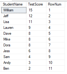
This is as simple as it gets, we’ve got a sequential number for each row.
With this function there’s no logic in here for handing any decision in the event of a tie. For this reason it can be helpful to have multiple fields in the ORDER BY to ensure uniqueness down to whichever level is required.
Rank
Next up we’ll look at the RANK function. The definition is very similar to the above function as it follows the anatomy we detailed above. The same example with RANK would look as follows:
SELECT *,
	[Rank] = RANK()
		OVER (ORDER BY TestScore DESC)
FROM #Students
ORDER BY 3;
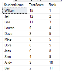
Whilst the definition may have been very similar the results have started to show the differences in these functions. Our records are still numbered 1 to 11 however we now have ties present which have the same Rank value.
The way in which RANK works is that any tie-breakers will be assigned the same ranking value, however the next values in the sequence will be skipped. Here we see the score of 8 is joint fifth for 3 students, so the ranks of 6 and 7 are skipped with the rank resuming at 8th position.
What about if we don’t want to skip those values from our ranking and we want it continuous though?
Dense Rank
The DENSE_RANK function is – as the name indicates – very similar to the RANK function above. This fills the gap left by that function (pun intended, apologies). Let’s use the same example again but with this function:
SELECT *,
	DenseRank = DENSE_RANK()
		OVER (ORDER BY TestScore DESC)
FROM #Students
ORDER BY 3;
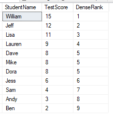
The output is similar to the RANK function, and the tie for fifth place still exists. Where this differs is that the sequence will be consecutive so won’t skip any ranking values – here we see the next record after the tie for rank 5 is rank 6.
This means our sequence is shortened from the ranking of 1-11 (with ROW_NUMBER and RANK) to be only 9 with this function.
NTILE
While the previous functions have been very sequential in nature, this function is a little different. This is designed to help segment data into a given number of equal(ish) groups. Let’s look at an example and then highlight the differences:
SELECT *,
	[NTile] = NTILE(4)
		OVER (ORDER BY TestScore DESC)
FROM #Students
ORDER BY 3;
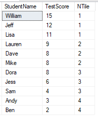
You’ll see immediately in the definition that this is the only function which takes a parameter. This is the number of groups we’re looking to create – 4 in this instance. This function isn’t strictly for ranking as we’d normally consider it however it has a similar idea of ordering so falls within the same category of functions.
In this example we’ve got 4 groups for 11 students which doesn’t fit well, so you’ll see the result is that we have the first three groups with 3 students and the fourth one only has 2. For uneven splits like this the earlier groups will have more than the later ones – imagine dealing a pile of cards out yourself.
Wrap up
Here we’ve looked at how ranking functions are defined proceeded with examples of each of them looking at how the outputs differ for them:
ROW_NUMBERto get a unique sequential rankRANKfor ranking with duplicate values for ties but a broken sequenceDENSE_RANKto provide duplicate ties but with consecutive unbroken sequenceNTILEfor distributing the results into groups
These functions are key to solving a variety of challenges when querying data, for example producing analytic or reporting data, or returning only portions of a dataset when performing paging or ranking.
If you’re looking to go a little further with ranking, these functions are also known as Window Functions as the ranking can be scoped to a specific window of data. An example of this could be if we had the class of the student included above and we could perform ranking within each class. If you’d like to see more about using them in this way check out this previous post for more details.
