A little while back we looked at an introduction to table partitioning where we covered the concepts involved in the partitioning. This time out we’ll look at how to implement those concepts to create a partitioned table.
As we’re going through the motions for this let’s start off by creating a table and fill it with some test data which we’ll then implement partitioning against:
/* Create the table */
CREATE TABLE SalesData (
	ID INT IDENTITY(1, 1),
	SalesDate DATE,
	SalesQuantity INT,
	SalesValue DECIMAL(9, 2)
);

/* Populate 100k random records */
WITH RandomData AS (

		SELECT 1 [Counter],
			DATEADD(DAY, CAST(RAND(CHECKSUM(NEWID())) * 10000 AS INT), '1999-01-01') [SalesDate],
			CAST(RAND(CHECKSUM(NEWID())) * 50 AS INT) [SalesQuantity],
			CAST(RAND(CHECKSUM(NEWID())) * 1000 AS DECIMAL(9, 2)) [SalesValue]
	UNION ALL
		SELECT [Counter] + 1,
			DATEADD(DAY, CAST(RAND(CHECKSUM(NEWID())) * 10000 AS INT), '1999-01-01'),
			CAST(RAND(CHECKSUM(NEWID())) * 50 AS INT),
			CAST(RAND(CHECKSUM(NEWID())) * 1000 AS DECIMAL(9, 2))
		FROM RandomData
		WHERE [Counter] < 100000
)
INSERT INTO SalesData (SalesDate, SalesQuantity, SalesValue)
SELECT SalesDate, SalesQuantity, SalesValue
FROM RandomData
OPTION (MAXRECURSION 0);
Creating a partition function
Our first step is to create a Partition Function. This is what will tell the engine how to split our data up and so the data type we use for it should align to one we’ve used in our table. Typically this is done in a way which logically splits the data into manageable buckets, for example it could be a DATE and we may split the data into quarters, or an INT which indicates a status so that we could manage active or historical data separately within the same table.
Based on our table design we’re going to choose to partition by the SalesDate field. The ranges which we’ll use for this would be annually. As a result this would allow us to manage each year of data individually if we needed to perform any maintenance or archiving on the data set.
When creating the function we have a choice of choosing RANGE LEFT or RANGE RIGHT for our partition values. This determines which bucket the data will be placed in depending on which side of the boundary they sit on. For example with a DATE boundary and values which include 1st February and 1st of March then for a RANGE RIGHT function any value which fell from 1st February to the right (imagine it along a timeline) prior to 1st March would fall under the 1st February partition. However if we used a RANGE LEFT function then anything after (but not including) 1st February up to (and including) 1st March would be included in the 1st March partition as it falls to the left of that boundary value.
Generally with DATE partition functions its more typically to see RANGE RIGHT as that ties up with how we think about time moving forwards from a given boundary value.
With those decisions made it’s now time for us to create our partition function. We’ll declare the DATE type and use RANGE RIGHT for the values, and then we’ll want to specify the initial boundary values to be used:
CREATE PARTITION FUNCTION MyPartFunc (DATE)
AS RANGE RIGHT
FOR VALUES ('2000-01-01', '2001-01-01', '2002-01-01', '2003-01-01', '2004-01-01', '2005-01-01', '2006-01-01', '2007-01-01', '2008-01-01',
	'2009-01-01', '2010-01-01', '2011-01-01', '2012-01-01', '2013-01-01', '2014-01-01', '2015-01-01', '2016-01-01',
	'2017-01-01', '2018-01-01', '2019-01-01', '2020-01-01', '2021-01-01', '2022-01-01', '2023-01-01', '2024-01-01');
That’s the most involved portion out of the way at least.
Creating the partition scheme
With our partition function in place we can now create a Partition Scheme. A partition scheme is needed to tie together the partition function which defines how we want to split our data, and our actual data which is what we want to be splitting up.
A partition scheme is used to map the partitions we’ve declared in our function to filegroups within a database. This can allow you to spread a partitioned table across multiple files which could even be located on different disks or tiered storage for example.
Using multiple filegroups is outside of the scope for this post, however this is an optional feature of the scheme. We can also choose to locate all our partitions inside the primary filegroup if that is our preference – which it will be in this example.
Creating our scheme is very straightforward as we’re keeping all the data together in the same (Primary) filegroup:
CREATE PARTITION SCHEME MyPartScheme
AS PARTITION MyPartFunc
ALL TO ([PRIMARY]);
With that in place we can finally get to actually splitting our data up.
Partitioning the table
To partition our table we need to apply the partitioning function (via the partition scheme) to our data. As we’re looking to split the underlying table this will need to be applied to the clustered index for the table, and this would then be known as an ‘aligned index’ as it aligns to a partition function.
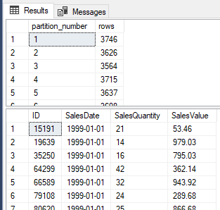
Before we do that however I just want to show a couple of snips of the data in its current state as a point of reference. Firstly we’ll look at the partitions currently showing for the table, and then look at the first few records in the table:
SELECT partition_number, [rows]
FROM sys.partitions
WHERE OBJECT_NAME(object_id) = 'SalesData';

SELECT TOP 100 *
FROM dbo.SalesData;

This shows us that we’ve got the singular partition for our data currently (its a heap) and we can see our data incrementing from our identity ID column as we’ve inserted it.
Conveniently for us we don’t yet have a clustered index on our table now so let’s see how the creation looks when its partition aligned:
CREATE CLUSTERED INDEX cx_SalesDate
ON dbo.SalesData (SalesDate)
ON MyPartScheme (SalesDate);
You’ll see that we’re not simply specifying the index on the table, but also that it’s on our partitioning scheme too. When the clustered index is created it’ll take the singular bucket of data we had before and carve it up into individual buckets for each partition which we’ve specified.
With that in place let’s rerun the same query from before and see how our data looks now:
SELECT partition_number, [rows]
FROM sys.partitions
WHERE OBJECT_NAME(object_id) = 'SalesData';

SELECT TOP 100 *
FROM dbo.SalesData;
Firstly we can see that we now have multiple partitions with the data spread out (mission accomplished!). What you’ll also see is that now that we’ve clustered (ordered) the data in this way, the start of our table is based on the date beginning from 1999 (our earliest entry) and not in the same order as it was inserted which we could see from the ID field previously.
Wrap up
As we mentioned in the initial post, partitioning is about the way that data is handled. We’re able to see benefits to the way that we manage and query our data through the use of effective partitioning strategies.
What we can see from our queries towards the end is that querying the table doesn’t change now that it’s partitioned. The way we design our partitions doesn’t need to impact the way we design our queries. It can however allow us to modify our queries or processes in different ways which may help to use the data more effectively if it’s designed well.
Hopefully this has given a good insight into implementing partitioning and I’ll look to follow up with some further details diving into various aspects of partitioning a little further.
