Last time out, following up to our posts looking at an introduction to partitioning and how to implement it we started to look at how to manage partitions.
In this post we’ll continue that theme by looking at how we’d go about removing (or merging) partitions as well as covering some general considerations when we’re performing operations on partitions and the tables they’re used by.
As usual we’ll start with a baseline which we’ve used with the previous examples:
/* Create a partition function to use */
CREATE PARTITION FUNCTION MyPartFunc (DATE)
AS RANGE RIGHT
FOR VALUES ('2000-01-01', '2001-01-01', '2002-01-01', '2003-01-01', '2004-01-01', '2005-01-01', '2006-01-01', '2007-01-01', '2008-01-01',
    '2009-01-01', '2010-01-01', '2011-01-01', '2012-01-01', '2013-01-01', '2014-01-01', '2015-01-01', '2016-01-01',
    '2017-01-01', '2018-01-01', '2019-01-01', '2020-01-01', '2021-01-01', '2022-01-01', '2023-01-01', '2024-01-01');

/* Create a partition scheme for the function */
CREATE PARTITION SCHEME MyPartScheme
AS PARTITION MyPartFunc
ALL TO ([PRIMARY]);

/* Create the table */
CREATE TABLE SalesData (
    ID INT IDENTITY(1, 1),
    SalesDate DATE,
    SalesQuantity INT,
    SalesValue DECIMAL(9, 2)
);

/* Apply clustering key */
CREATE CLUSTERED INDEX cx_SalesDate
ON dbo.SalesData (SalesDate)
ON MyPartScheme (SalesDate);

/* Populate 100k random records */
WITH RandomData AS (

        SELECT 1 [Counter],
            DATEADD(DAY, CAST(RAND(CHECKSUM(NEWID())) * 10000 AS INT), '1999-01-01') [SalesDate],
            CAST(RAND(CHECKSUM(NEWID())) * 50 AS INT) [SalesQuantity],
            CAST(RAND(CHECKSUM(NEWID())) * 1000 AS DECIMAL(9, 2)) [SalesValue]
    UNION ALL
        SELECT [Counter] + 1,
            DATEADD(DAY, CAST(RAND(CHECKSUM(NEWID())) * 10000 AS INT), '1999-01-01'),
            CAST(RAND(CHECKSUM(NEWID())) * 50 AS INT),
            CAST(RAND(CHECKSUM(NEWID())) * 1000 AS DECIMAL(9, 2))
        FROM RandomData
        WHERE [Counter] < 100000
)
INSERT INTO SalesData (SalesDate, SalesQuantity, SalesValue)
SELECT SalesDate, SalesQuantity, SalesValue
FROM RandomData
OPTION (MAXRECURSION 0);
Removing a partition
We may occasionally have need to remove partitions from our partition function. This may be that we’ve had the profile of the data change or we could have partitions which are too granular and need combining for example.
Removing a partition doesn’t remove the data held within that partition. When we remove a partition we’re actually merging that partition with anther. The data will be merged into an appropriate adjacent partition. If the partition function is RANGE LEFT then removing a partition would move the data into the partition to the right, and similarly for a RANGE RIGHT function this would move the data into the partition to the left.
Let’s see an example of it in action. We’ll start by taking a look at the number of records in each of our partitions to start with:
SELECT partition_number, [rows]
FROM sys.partitions
WHERE OBJECT_NAME(object_id) = 'SalesData';
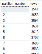
Lets bear in mind that we’re using a RANGE RIGHT for our function so we’ll have partition 1 storing any data prior to our first boundary value, then partition 2 which stores from our first boundary (January 2000) until the boundary value for partition 3 (January 2001).
In our example we’ll remove the boundary for January 2001 which is partition 3 in this screenshot. All of those values will be dated to the right of our partition 2 boundary which is January 2000, and to the left of our partition 4 which is January 2002. As we’re using RANGE RIGHT they will move to the left into the existing partition 2.
We can now go ahead and remove the partition as follows:
ALTER PARTITION FUNCTION MyPartFunc()
MERGE RANGE ('2001-01-01');
With the operation complete we can see how the partitions look following this change:

As expected we can see that the number of records for partition 2 have increased to include the records which were previously in partition 3. You can also see that the partition numbers have adjusted to maintain a continuous sequence rather than leaving a gap without partition 3 present.
It’s worth noting here that similar to when we were splitting partitions it can be quite a resource intensive operation to remove a partition. This is due to all of the data needing to be rewritten into a different partition so the timing and volume of records for these operations should be considered.
Considerations
When we’re managing partitions we’re changing where data is being stored which means that it can be quite costly to perform these operations as noted above. There are a couple of considerations I wanted to touch on around these types of maintenance operations.
Large numbers of changes
Performing a large number of the operations we’ve discussed recently may be very time and resource intensive as they’re all separate operations on the data. You can’t create or merge multiple partitions in a single operation, and each addition or removal could require a chunk a data being rewritten.
There are a few ways which could be considered to alleviate the impact of these:
- Ensure partitions are empty if possible before maintenance is performed on them. For example if you have an empty partition at the end of your function then splitting it down will be much faster due to not having to rewrite data. Of course this option may not always be available.
- Schedule or stagger the changes to minimise impact rather than making all of the changes in a single batch which would cause blocking a require a large amount of resources for an extended period. Again this may not be feasible depending on the volume of changes or the timescale needed.
- Recreate the partition function, schema and table and gradually move data into the new table from the old one. This will alleviate any work on the existing table and the partitions for the new table will be created as data is inserted. Once all the data is migrated the tables can be renamed to switch the old and new tables.
These options all have their own advantages and disadvantages which will largely come down to the volume of data you’re dealing with and what impact or downtime may be available to you when completing the work.
The last point can be preferable when you want to minimise impact on an existing table so long as you have sufficient storage to store twice the volume of data for a period whilst you transition it. This can also be the cleanest as you’ll choose what data to rewrite as you copy it across rather than being forced to rewrite entire partitions when splitting or merging them.
Sharing partition functions
We’ve seen previously that we create a partition function, the scheme and then the table. As these are layered on top of each other we could use the same partition scheme for multiple tables, or the same partition function for multiple schemes and tables.
Whilst we can do that however, it’s not always the best way to approach partitioning a set of data. The reason for this is that if we have a few tables all partitioned using the same function and we want to make a change to our function we may come up against two challenges:
- We can’t choose to only separate or merge a partition in one table, it would take place in all of them as they share the function
- The operation would be performed on all tables at the same time which could take a lot of time and resources depending on the (combined) size of the tables and partitions which are using that function
This may not be so much of an issue in a well established and maintained data set, however in more infant or fluid environments this can become a challenge. It can be beneficial to use separate functions and schemes for at least the largest of tables due to this.
Wrap up
We’ve followed up on our previous post talking about splitting and adding partitions by discussing how to merge and remove partitions. We’ve also continued to look at a couple of considerations when managing partitions, particularly in environments with larger volumes or data.
The subject of partitions has a very wide scope and I’ve got some more ideas for how we can take this further. Is there anything more you’d like to see in this area or any other in particular?
