T-SQL Tuesday #168 – Mature Window Functions

This month’s invitation from Steve asks us to about how window functions have made life easier for us. Before we get into that let’s have a brief recap of what window functions are for those who aren’t familiar.

What are they?

Window functions are like regular functions we’d use in a result set such as SUM() or MIN() but more powerful. The regular functions get applied against the data in our tables. Window functions are relative to the results returned. You can think of these as a sort of post-processing.

So to the first question of the day: How have they made life easier?

Window functions can help us simplify queries. We can use them in situations that would otherwise need self joins or a CTE. This makes it not only quicker to define, but also makes the resulting query much easier to read.

That’s the easy part out of the way, now let’s look at them in action.

Setting up

Before we jump in we need some sample data to play with. Below are some fake monthly sales for a couple of years in a temp table which we’ll use:

CREATE TABLE #MonthlySales (
    FinancialYear CHAR(6),
    FinancialQuarter CHAR(7),
    FinancialPeriod CHAR(7),
    SalesValue MONEY
);

INSERT INTO #MonthlySales
VALUES ('FY2021', '2021Q01', '2021P01', 1700.99), ('FY2021', '2021Q01', '2021P02', 2.29), ('FY2021', '2021Q01', '2021P03', 9.99), ('FY2021', '2021Q02', '2021P04', 1214.85), ('FY2021', '2021Q02', '2021P05', 2049.10), ('FY2021', '2021Q02', '2021P06', 3.99),
	('FY2021', '2021Q03', '2021P07', 54.99), ('FY2021', '2021Q03', '2021P08', 24.49), ('FY2021', '2021Q03', '2021P09', 2181.56), ('FY2021', '2021Q04', '2021P10', 564.99), ('FY2021', '2021Q04', '2021P11', 699.09), ('FY2021', '2021Q04', '2021P12', 53.99),
	('FY2022', '2022Q01', '2022P01', 29.99), ('FY2022', '2022Q01', '2022P02', 7.95), ('FY2022', '2022Q01', '2022P03', 21.49), ('FY2022', '2022Q02', '2022P04', 769.49), ('FY2022', '2022Q02', '2022P05', 21.98), ('FY2022', '2022Q02', '2022P06', 539.99),
	('FY2022', '2022Q03', '2022P07', 3399.99), ('FY2022', '2022Q03', '2022P08', 32.60), ('FY2022', '2022Q03', '2022P09', 49.99), ('FY2022', '2022Q04', '2022P10', 1000.43), ('FY2022', '2022Q04', '2022P11', 742.35), ('FY2022', '2022Q04', '2022P12', 4.99);

With that created we can look at the main takeaway for today: What problems can we solve with them?

The functions relate to ranking, aggregation and analysis. There can be some use for these in operational systems, however my main go-to for these functions is with data analysis.

I wanted to take a look at a couple of scenarios we can demo with the data above.

Relative averages

The first situation is looking at averages. For our data set we’ll look at the average for the quarter as well as a rolling average for three periods.

We achieve a quarterly average with the PARTITION clause for the function. This clause defines how we’ll split our data before applying the function. In this case we’ll split it by the quarter. The AVG function will then apply across any rows which have the same quarter as we’re returning.

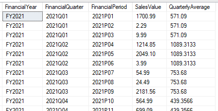
It’s easier to see it in action. Here are the results:

SELECT
	s.*,
	QuarterlyAverage = 
		AVG(SalesValue)
		OVER (PARTITION BY FinancialQuarter)
FROM #MonthlySales s;

We can see the average calculated is consistent and correct for each quarter in our data. Great, let’s try another example.

This time we’ll look at a rolling average for the last 3 periods. As a rolling period applies to all rows we won’t be partitioning this time. We’ll use the ROWS clause to define relative rows in the results. This will also depend on the use of an ORDER BY clause to make sure the periods are in the correct order.

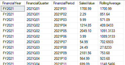
This is how the query and results look:

SELECT
	s.*,
	RollingAverage = 
		AVG(SalesValue)
		OVER (ORDER BY FinancialPeriod
		ROWS BETWEEN 2 PRECEDING
			AND CURRENT ROW)
FROM #MonthlySales s;

We specified 2 preceding rows up to the current row to provide the average across 3 periods. It is key that we specify an order to make sure the preceding rows are the ones we expect. We see the first two rows only have one or two records to average. When we get down to the 3rd row onwards we have enough data to perform the full rolling average.

We’ve looked at averages here but you can apply the same to a variety of other window functions. I’ll pop some references to these at the end of the post.

Relative performance

Next up we’ll take a look at relative performance. This uses one of the analytical functions – LAG. Steve mentioned we’ll get bonus points for this so how could I not include it.

The LAG function returns a value from a preceding record based on the ORDER BY. We can choose how far behind the current record based on a parameter.

That’s right, this function takes multiple parameters. The parameters we have are for: the value we want to display, the number of records behind to go, and a default value.

Let’s take a look at the query and we’ll discuss it after:

SELECT
	s.*,
	PreviousPeriod =
		LAG(SalesValue, 1, 0)
		OVER (ORDER BY FinancialPeriod),
	PreviousQuarter =
		LAG(SalesValue, 3, 0)
		OVER (ORDER BY FinancialPeriod)
FROM #MonthlySales s;

We’ve got two examples here to show how it works. Firstly the parameters. We’ve got a lag values of 1 and 3 to show results from the previous period and quarter. We also use a default value of zero but could have used SalesValue (for the current row) if preferred.

You’ll see for the first row that as we don’t have previous rows to refer to they have fallen back to the default value. This also continues for rows 2 and 3 which don’t have a previous quarter to refer to.

Let’s have another quick example to show how window functions work. This follows on from the query above with a WHERE clause added:

SELECT
	s.*,
	PreviousPeriod =
		LAG(SalesValue, 1, 0)
		OVER (ORDER BY FinancialPeriod),
	PreviousQuarter =
		LAG(SalesValue, 3, 0)
		OVER (ORDER BY FinancialPeriod)
FROM #MonthlySales s
WHERE s.FinancialQuarter = '2021Q02';

Hmm, that’s a little different. We’ve lost some of those values we had last time. How come?

Remember when we started by saying that window functions are post-processing for our data? – that’s what has happened here.

The window functions are being applied after the filtering has taken place. This means we don’t have the previous records which the LAG function would have picked up. It’s a nuance of window function we need to understand to be able to use them effectively.

Query plans

The last part I wanted to touch on was the query plans produced by these functions. Earlier I mentioned that these can save you from needing to use a CTE or a self join.

We’ll go back to our quarterly average query from earlier and reconstruct that as a CTE:

WITH AverageCTE AS (
	SELECT FinancialQuarter, QuarterlyAverage = AVG(SalesValue)
	FROM #MonthlySales
	GROUP BY FinancialQuarter
)
SELECT m.*, c.QuarterlyAverage
FROM #MonthlySales m
	INNER JOIN AverageCTE c ON m.FinancialQuarter = c.FinancialQuarter;

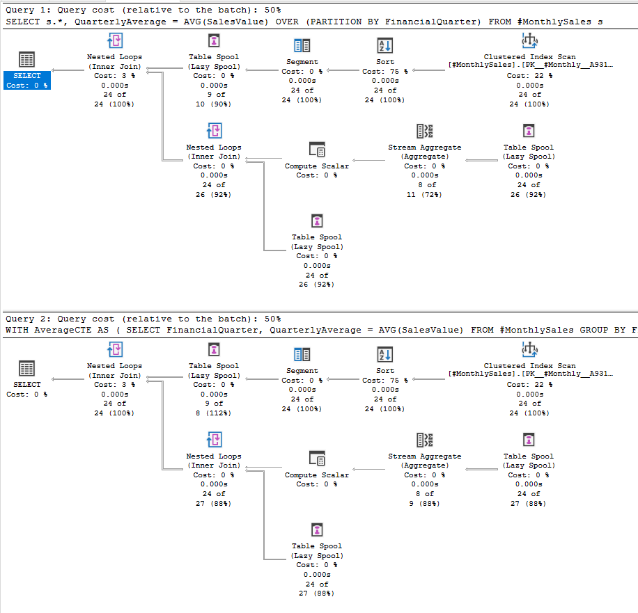
The data returned is the same as our previous query. The definition is a bit more verbose, but how does it perform?

The statistics for this showed both plans performing 83 logical reads – 81 for a work table and 2 for our temp table. We can see that the optimiser implements this in a similar what to what we can.

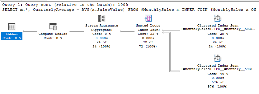
It’s not too bad of an implementation. How about the same with a self join though?

SELECT
	m.*,
	QuarterlyAverage = AVG(x.SalesValue)
FROM
	#MonthlySales m
	INNER JOIN #MonthlySales x
		ON m.FinancialQuarter = x.FinancialQuarter
GROUP BY
	m.FinancialYear, 
	m.FinancialQuarter, 
	m.FinancialPeriod, 
	m.SalesValue;

This gives us a much tighter plan than the previous examples. We also don’t need a work table in this case. Our logical reads drop to 51 and are all from our temp table.

In this instance the window function may not provide the absolute best performance. It works well enough for our limited sample data though. Everyone’s data set will be different. It’s worth exploring an alternative approach on your data to see how it compares to a window function.

Wrap up

This post is getting onto the longer side for me so let’s wrap it up.

Today we’ve looked at where data analysis can benefit from use of window functions. They help our queries to be more concise. We’ve touched on nuances and gotchas with window functions too.

Window functions are another tool we have to change how we do what we do. It doesn’t change what we can return but it’s an other option for how we return it. It helps with clarity and can remove instances of death-by-CTE.

If you’re new to CTEs then you’re in luck with this month’s T-SQL Tuesday ask from Steve. There will be some great responses from across the community, enjoy!

We’ve looked at Window Functions on the blog before if you’d like to dive into those further. Here are some specific posts related to ranking, aggregates and analytical functions.