Anatomy of a Window Function Execution Plan

After last week’s post I got to thinking that although we’ve looked at how to implement window functions, we haven’t peeked under the hood to see how they are executed.

Then what do you know, Kevin has picked up my post to provide an alternative approach. He observed that whilst his approach was more straightforward it produced a more complex execution plan.

As Kevin pointed out, using different approaches will lead to different execution plans. Depending on the shape of our data we may prefer one approach over another due to the plan produced. By understanding the operators which are used to apply the functions we can make more informed decisions as to which approach we’d prefer.

Using last week’s sample data we can run the query below to demonstrate operators typically used for a window function:

SELECT *,
    SUM(SalesValue)
        OVER (PARTITION BY FinancialQuarter
                ORDER BY FinancialPeriod)
FROM #MonthlySales;

The result of this query is a set of data with a running total of the Sales Value within each Financial Quarter.

We’ll follow the data through some of the operators in this execution plan to understand their part in the function. As with regular execution plans we’ll be working from right to left.

Sort

We’re used to seeing the sort operator in our queries. The difference we’ll see with window functions is that the operator will be earlier in the plan than we may usually see.

The reason for it being earlier in this plan is that we need our data sorted before we can start to build our windows to apply the SUM operation against.

A typical Sort will order the data based on the ORDER BY clause specified, but there’s more to them with Window Functions. This sort operator is sorted based on both the field we’re ordering by, as well as the field we’re partitioning by:

The reason for sorting our partition field is due to our next operator.

Segment

The Segment operator is used to detect changes in our data and to segment it up in preparation for our window function. This operator looks for changes in our data from row to row to help define segments in our data. As we’re using both PARTITION BY and ORDER BY clauses in our function we require two of these.

The first operator will segment the data based on our PARTITION BY clause, the Financial Quarter in this case. The properties for the operator show a new field being output (‘Segment1007’ in our case) which will indicate which partition is in each segment:

Once that has been processed our second Segment operator will deal with our ORDER BY clause and segment data based on the Financial Period. We can see this in the properties for the operator, with this segment being output as add additional (‘Segment 1008’ in our query):

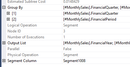
These second segments will identify the change in the ORDER BY fields (our Financial Period) which will facilitate the running total being applied against current and previous Periods within the Quarter.

The segment steps are preparation to analyse our data ready for performing the windows and aggregation. So it’s onward to our next operator…

Window spool

The Window Spool operator is the one which does the ‘windowing’ process for our function. I’ll use the term ‘window’ to mean the set of rows which the function will be applied against to return a value for each row in our result set.

This operator will work through the data row by row. It uses the segments defined previously to gather rows which are in the same window as the record being processed. Being a spool, this works by caching the data in each partition as rows can be reused for subsequent windows if applicable.

Once the operator has identified all of the rows for a particular window it will send them onward. The output for this function contains the segments defined previously but will also include a new field to identify which window the row belongs to (‘WindowCount1009’ in this example):

If you’d like to read more about this operator (as well as any others) there’s a great resource on SQLServerFast with much, much more detail.

Depending on our query we can also see Table Spool or Index Spool operators. These instances will cache a larger set of data and will typically be integrated into the function via a JOIN operator.

Now that we’ve segmented our data and defined the records in the window there’s only one part left…

Stream aggregate

The Stream Aggregate operator is when we finally get to applying the function to our data. This is the same operator we’d see when performing aggregations usually.

In this instance however we aren’t performing an aggregate with a GROUP BY operator. We are grouping all the records provided by the Window Spool which fall within the same window. This is shown by the operator grouping based on the field output by our spool above:

As with other aggregations this operator will perform the required function (SUM in this case) as well as a COUNT. The result of the count will be used by the following Compute Scalar to determine whether to display a value or NULL result.

Wrap up

In this post we’ve looked at the operators used to build a straightforward Window Function. These are operators which you might not see often outside of these functions such as Segment or Window Spool. Others are more common operators which may behave a little differently in the context of a Window Function such as the Sort operator.

We’ve covered each operator and their purpose in the execution plan. These aren’t the only operators you’ll see in the plan which uses a window function. You will see these and a variety of more standard operators such as Table Spools or Join operators. The complexity of the plan will depend on your data and query.

Hopefully this helps folks understand what they’re seeing when looking at plans involving a Window Function. Knowing how the operators are needed when looking at a plan can help us to understand how results are derived and where opportunities may be to make these queries more efficient.