
In Synapse SQL Pools, Hash distributions allow us to somewhat control data distribution. Whilst this can deliver performance in the right scenarios, I noted last week that these tables should be monitored to avoid skew.
In this post I want to demonstrate how to identify the skew, and why a different distribution model may be better suited.
Issues with skew
As a recap from last week, each table is divided across 60 distributions, which are our query processors. Ideally we want an even spread of rows across each distribution to balance processing.
Hashing divides rows across distributions based on the hashed value of a field, so the values in that field determine the spread.
The skew is caused when the hash results in unbalanced distributions. This impacts performance due to some distributions being heavily loaded and others having minimal or no work to do, which creates a bottleneck on the larger distributions. You can think of this like unbalanced parallelism in SQL Server.
Identifying skew
Monitoring for skew is key to ensure our distribution approaches are providing even coverage across distributions. For Replicated and Round Robin tables, this isn’t usually an issue.
This query uses DMVs to return table metrics, including skew:
WITH TableDistributions AS (

    /* CTE handles partitioned tables */
    SELECT
        SchemaName = s.[name],
        TableName = t.[name],
        DistributionPolicy = tp.distribution_policy_desc,
        nt.distribution_id,
        DistRows = SUM(nps.row_count),
        DistSizeMb = SUM(nps.reserved_page_count) * 8 / 1024.0
    FROM
        sys.tables t
        INNER JOIN sys.schemas s ON t.[schema_id] = s.[schema_id]
        INNER JOIN sys.indexes i ON i.[object_id] = t.[object_id] AND i.index_id <= 1
        INNER JOIN sys.pdw_table_distribution_properties tp ON tp.[object_id] = t.[object_id]
        INNER JOIN sys.pdw_table_mappings tm ON tm.[object_id] = t.[object_id]
        INNER JOIN sys.pdw_nodes_tables nt ON nt.name = tm.physical_name
        INNER JOIN sys.dm_pdw_nodes_db_partition_stats nps
            ON nps.[object_id] = nt.[object_id]
            AND nps.pdw_node_id = nt.pdw_node_id
            AND nps.distribution_id = nt.distribution_id
            AND nps.index_id = i.index_id
    GROUP BY
        s.[name],
        t.[name],
        tp.distribution_policy_desc,
        nt.distribution_id
)
SELECT
    SchemaName,
    TableName,
    DistributionPolicy,
    TotalRows = SUM(DistRows),
    MinRows = MIN(DistRows),
    MaxRows = MAX(DistRows),
    AvgRows = AVG(DistRows),
    MaxDistSkew = CAST(MAX(DistRows) * 1.0 / NULLIF(AVG(DistRows * 1.0), 0) AS DECIMAL(10,2)),
    ReservedSizeMb = CAST(SUM(DistSizeMb) AS DECIMAL(18,1))
FROM
    TableDistributions
GROUP BY
    SchemaName,
    TableName,
    DistributionPolicy
ORDER BY
    TotalRows DESC;
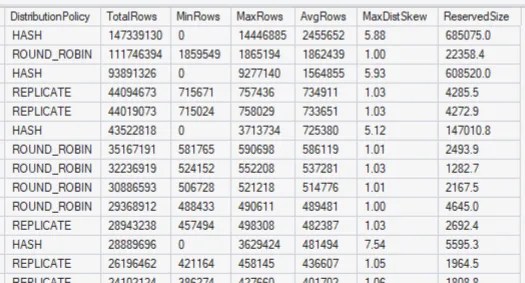
A skew value close to 1 indicates record counts are relatively even across distributions. A skew value of 5.88 shows the largest distribution has 5.88x the number of records of the average. The minimum and maximum row counts demonstrate the breadth of skew. Generally, a skew up to 1.1 won’t have a noticeable impact on performance.
For tables where we want to dive into a larger skew, we can use the following DBCC command:
DBCC PDW_SHOWSPACEUSED('dbo.MyHashTable');
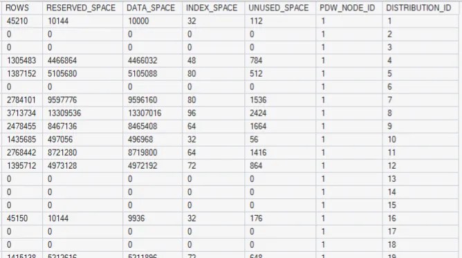
This provides the details across all of the distributions, and in this case a very feast-or-famine distribution.
Alternatives
The choice between two common alternatives boils down to a simple question: are there other related tables which share the same hash distribution?
1️⃣ If the Hash distribution is required for performance, such as joining two large fact tables, the alternative would be to include another field in the hash key to bring more uniqueness to the hashing. Let’s say you were joining by Month and Client, but only hashing by Month which produced an uneven distribution. Changing the hash to include the Client would provide more uniqueness and likely improve data distribution, whilst still mirroring the join conditions. To maintain performance, the joined tables would need the same hash key too.
Note that multi-column hashing needs to be enabled by setting database compatibility level to 50 – details here.
2️⃣ If Hash distribution is not required, then the simple alternative is to change to a Round Robin approach which will evenly distribute records when the table is populated. Depending on the reason the hash key was chosen, you might find it better suited as a clustered (rowstore) key with this type of distribution. The trade-off here is that it may cause additional data movement during joins, so understanding query patterns is key to validate before and after performance.
Now, you can’t change distribution on the fly, so you’ll need to create a new table using CTAS. Whilst this will take time and duplicate storage, it does allow you to rerun distribution checks against the new table to see the impact – particularly useful if you’re moving to a different field combination for hashing to ensure the rows are more balanced.
Wrap up
In this post we’ve moved from why distribution matters to what can happen when distribution goes awry. Skew is the gotcha for Hash distribution and is why these tables should be monitored.
Identifying and drilling into the skew is simple. Deciding if it needs to be tackled – and how – is the challenge. We’ve looked at two approaches here which solve it in different ways. The necessity of recreating tables makes it a no-brainer to perform side-by-side comparisons of the impact on both the skew and queries, before we commit to switching the tables out.
With 60 distributions in play we want an even spread to make sure they’re all pulling their weight. Skew is the kryptonite to this, so keep an eye out for it, or those heavier distributions can slowly become your bottleneck.

